Depth estimation and segmentation for 3D object tracking
This blog post explains how we fuse YOLO and MiDaS to perform 3D object tracking with monocular cameras.

By Christian Stippel
Object Positioning
In this post we explain how to obtain the 3D position bounding box of objects from monocular images by fusing the object detection algorithm You Only Look Once (YOLO) and depth estimation with deep learning. We show our evaluation of depth estimation models, explain how you can calibrate inverse depth maps and finally combine depth estimation with YOLO to obtain the spacial properties of objects.
Monocular Depth Estimation
We assume to have a static monocular image stream as input. Structure from motion cannot be used to obtain depth values because the camera is static. To obtain objects’ positions, we use absolute monocular depth cues encapsulated within neural networks.
Within our research, we found two types of depth estimation models:
- Absolute scale depth estimation produces depth values that need to be scaled if the underlying model was trained on data with different internal calibration.
- Inverse depth estimation, whose output must be scaled, shifted and inverted on a frame to frame basis.
We select AdaBins and MiDaS, because they have the highest accuracy on the NYU V2 dataset. AdaBins produces absolute depth maps, while MiDaS produces inverse depth estimations.
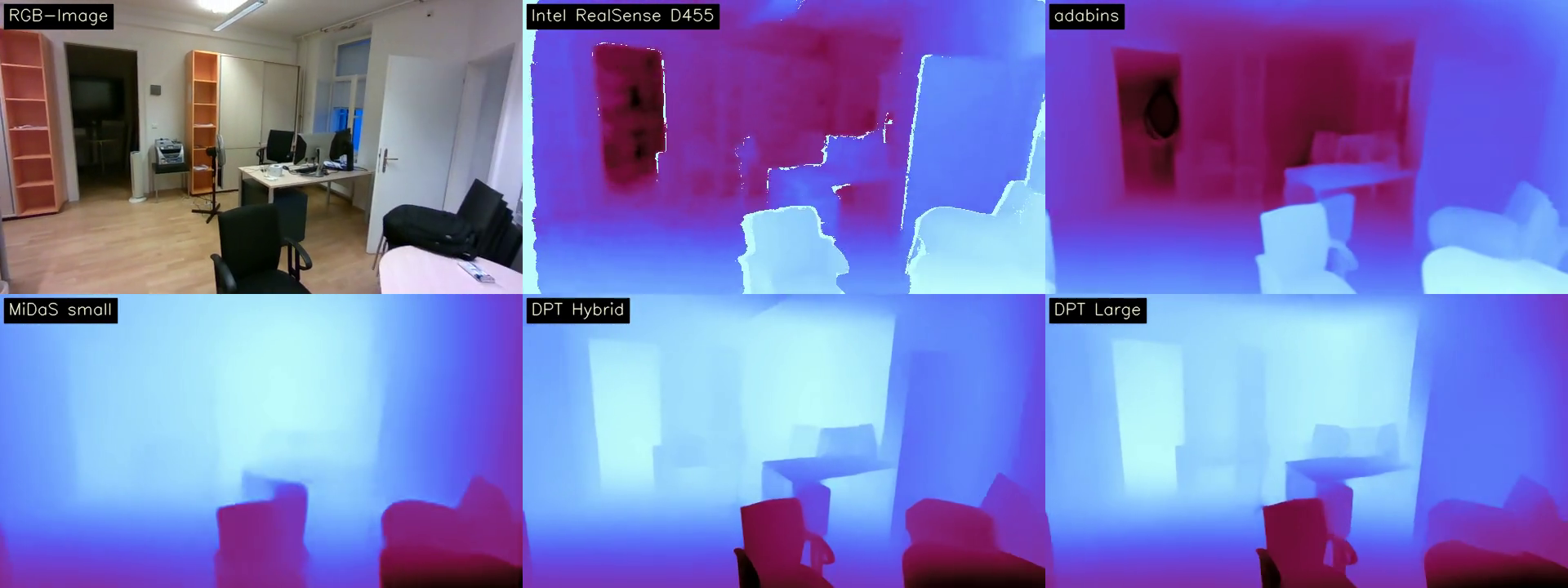
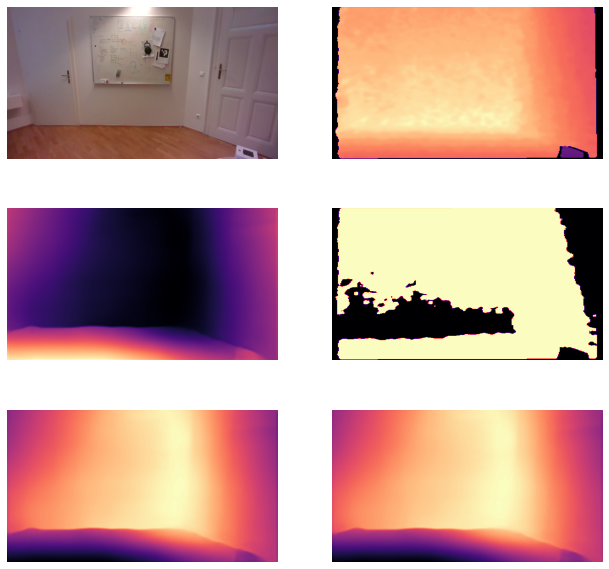
We evaluate the performance in regards to precision and inference time. Since the benchmarked models are trained on various depth data sets like ReDWeb, NYU Depth Dataset V2, etc. we created our own data set for benchmarking purposes to prevent any information leakage. We use an Intel RealSense Depth Camera D435, a stereo camera with prior known focal length and baseline, to record the RGB values and the absolute depth map of an image. An example of a side-by-side comparison of the different models as well as the ground truth images (RGB and depth) is displayed the following figure. The result color of MiDaS networks is inverted since they produce the inverse depth up to a scale and shift.
In order to evaluate the performance of the various models we use the RMSE. This metric is defined by:
\begin{equation} \sqrt{\frac{1}{|N|} \sum_{i \in N} ||y_i - \hat{y}_i||^2} \end{equation}
where $y_i$ is the measured ground truth depth value of pixel $i$ and $\hat{y_i}$ the corresponding predicted depth. Moreover, $N$ denotes the set of indices of all pixels of a given image and $|N|$ the cardinality of this set. For inference time we measured the time in seconds.
We find the RMSE and inference time and compare them. The images with an RMSE of 1 or higher are filtered out since they come from scene transitions and are thus not representative of the validity of the depth estimation. Furthermore, we scale the AdaBins depth estimation and find the scale and shift for MiDaS by using Least Squares with the corresponding stereo depth for MiDaS to scale the inverted and shift the depth values and invert them afterward.
We show the performance for single images and the overall performance across all images in the next images.
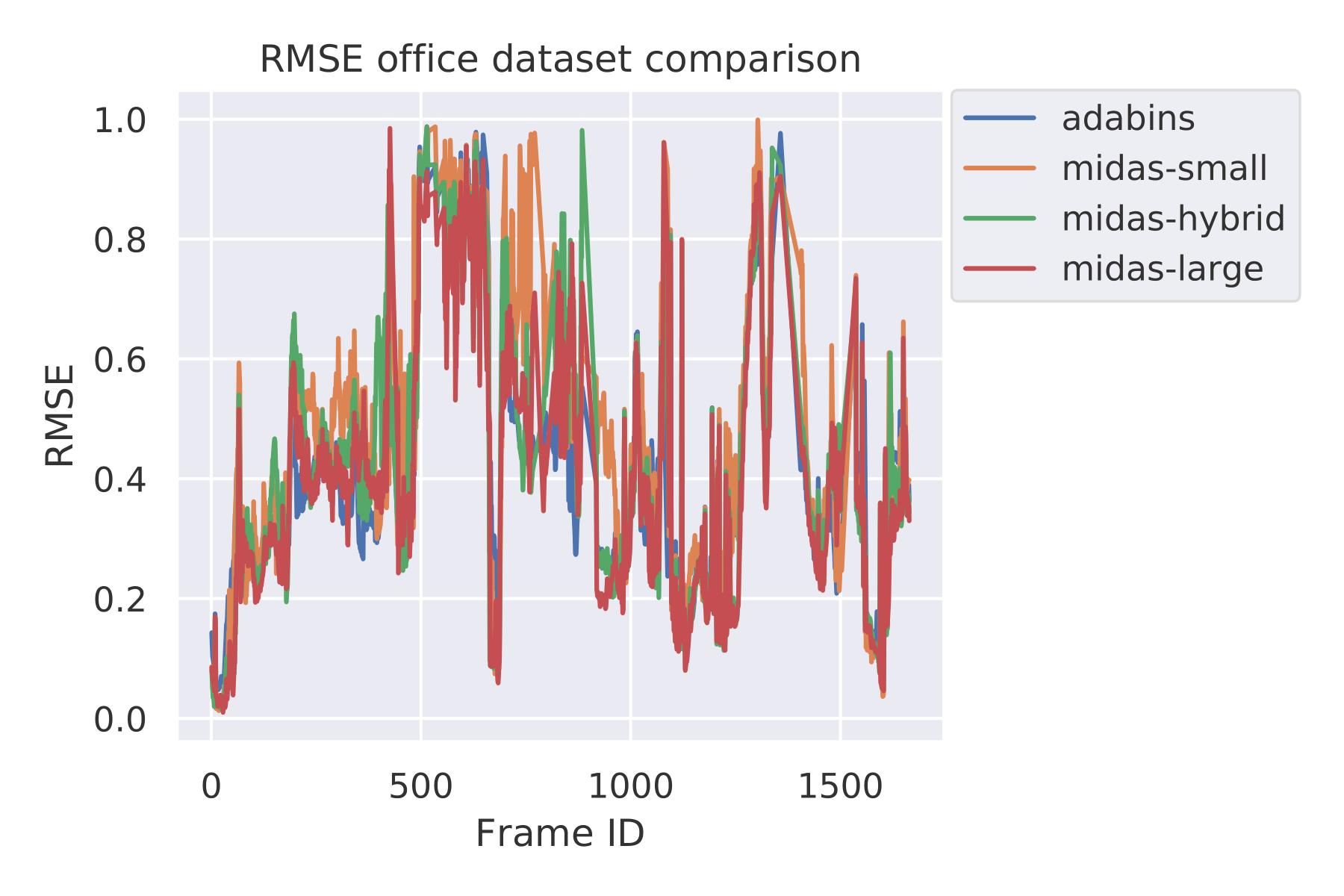
Interestingly, we can see that the performance of MiDaS large and AdaBins is very similar. AdaBins is slightly more stable across the time-lapse of the different images, and a higher relative standard deviation is occurring within the MiDaS models.
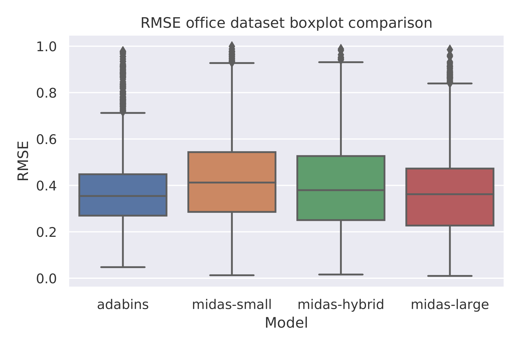
Here are the bencharking results of examined models on our dataset:
| Model | RMSE (mean) | RMSE (sd) |
|---|---|---|
| AdaBins | 0.388946 | 0.184682 |
| MiDaS small | 0.435106 | 0.214792 |
| MiDaS hybrid | 0.401826 | 0.210238 |
| MiDaS large | 0.375846 | 0.202608 |
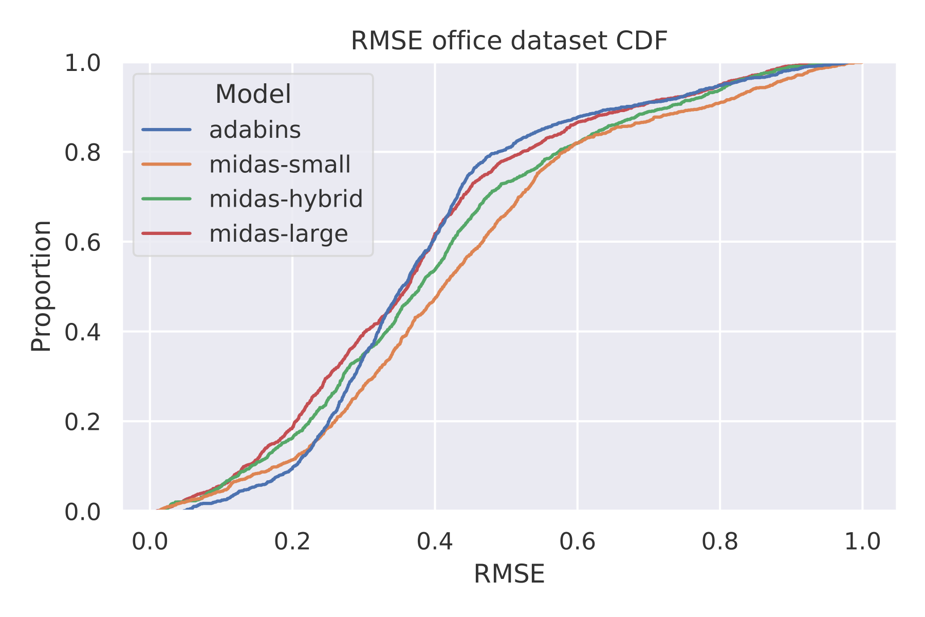
The cumulative distribution function (CDF) calculates the probability that a random observation will be less than or equal to a particular value. The next images show the CDF plots of our Office data set. We compare the precision of each network quantitatively here:
The next image shows the CDF of the inference time. We see that only the small version of MiDaS can evaluate multiple frames per second.
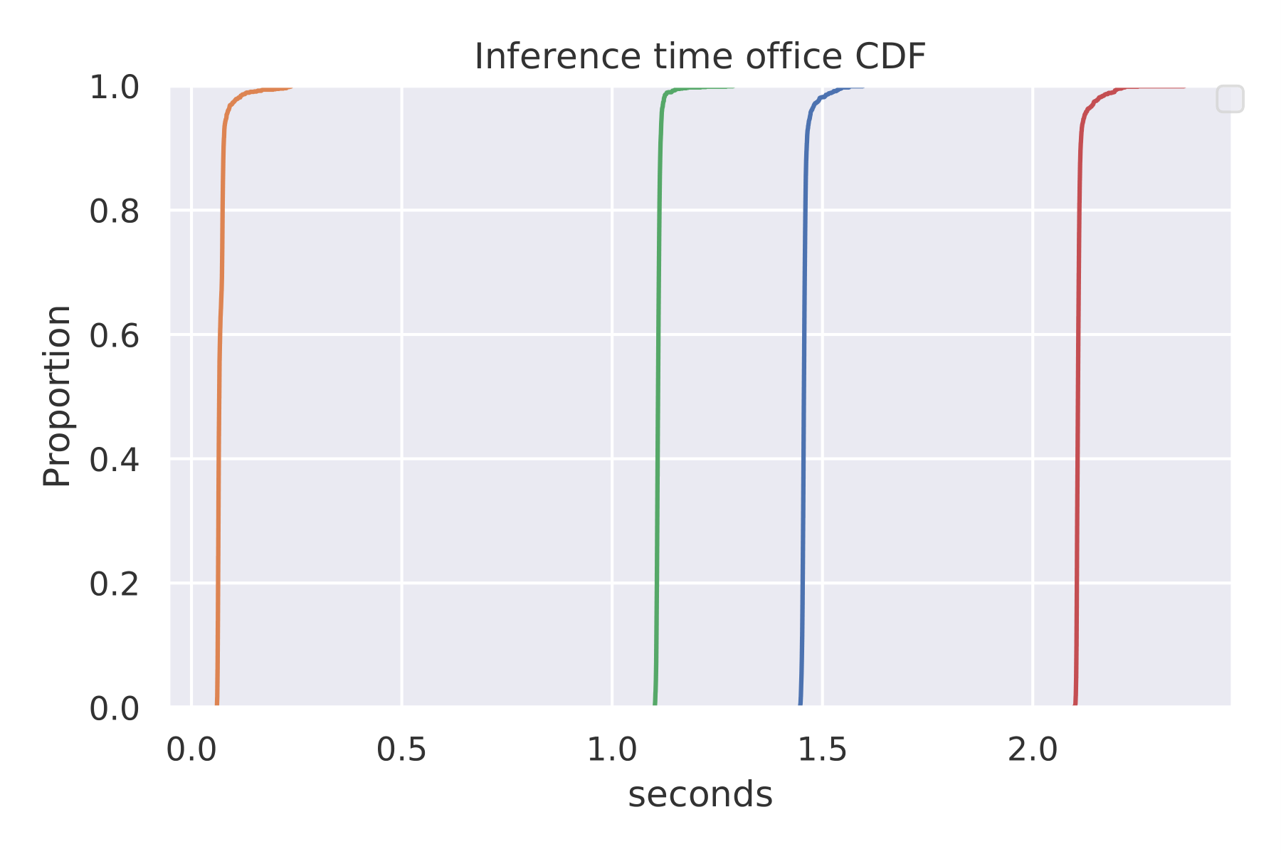
Since we want to estimate the position of objects in a real-time manner, we use the small version of MiDaS for depth estimation in subsequent sections.
Inverse Depth Mapping
MiDaS produces inverse depth values up to a scale and shift. Therefore we cannot use the raw output of MiDas for absolute scale position estimation. To calibrate the estimated inverse depth, we must find and apply the scale and shift of the depth values and invert them to obtain depth values in meters.
We present an algorithm to find the scale and shift robustly based on Random sample consensus (RANSAC). As input, we have an inverse depth estimation, up to a scale and shift, from MiDaS and an absolute depth map, which contains at least two depth values.
- We sample at least two depth values and calculate the scale and shift using least squares.
- The depth values are scaled, shifted, and inverted to obtain absolute depth values in meters.
- The calibrated estimated depth is compared to the absolute depth map.
- If a calibrated estimated depth value is less than 0.1 (10 cm) apart of the corresponding absolute depth value, it is labeled as an inlier. Otherwise, we label it as an outlier.
- We repeat steps 2-4 to maximize the number of inliers until a stopping criterion is met.
For the first RGB frame, we obtain the depth estimation with a pre-trained MiDaS small neural network. We use stereo vision to obtain absolute depth values and calibrate the depth estimation with the previously explained algorithm. The next image visualizes the calibration process.
For subsequent frames, we estimate the depth using MiDaS small and use the initial calibrated depth estimation as a reference to calibrate the depth estimation.
Fusing Object Detection and Depth Estimation
We find objects of interest with the object detection algorithm You only Look once (YoLo). YOLO maps images to 2D bounding boxes, labels, for example, “chair” or “person”, and a confidence value.
We can map each image point with a defined depth value to world coordinates by multiplying the corresponding ray with the absolute depth value and subtracting the camera position. We use a cuboid as a bounding box for objects. We assume that the front of the cuboid is orthogonal to the view ray. By mapping the center of the 2D bounding box to the corresponding 3D coordinates, we obtain the 3D front face of the bounding box. The other sides of the cuboid are obtained by assuming that the front is orthogonal to the camera’s view ray.
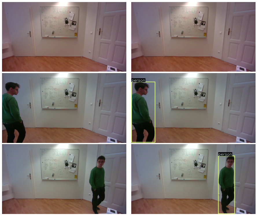
Let’s look at an example of an image stream with a person moving through the scene.
The top left image shows the resulting position and 3D bounding box. The top right shows the stereo depth generated by the Intel RealSense camera. The stereo depth is not used and is only shown as a reference for qualitative evaluation. As can be seen in the bottom left, the person is correctly masked. Therefore, moving objects are not used for calibrating the inverse depth. They are masked because the calibrated depth values of the current frame are more than 10 cm apart from the initial calibrated depth estimation since MiDas is consistent enough in predicting relative depth values.